Controllability and Observability
More specially, for system of Eq.(1), there exists a similar transformation that will diagonalize the system. In other words, There is a transformation matrix Q such that
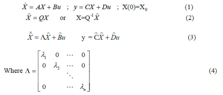
Notice that by doing the diagonalizing transformation, the resulting transfer function between u(s) and y(s) will not be altered.
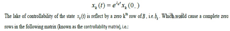
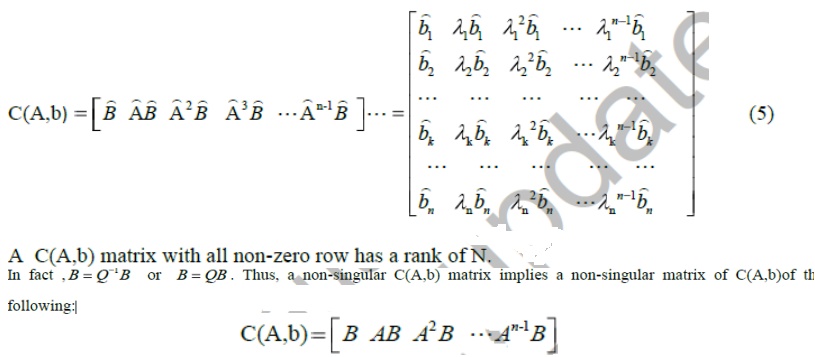
Looking at Eq.(3), if equ =0 is uncontrollable by the input u(t), since, xk(t) is characterized by the mode by the equation.
Transfer function from State Variable Representation
A simple example of system has an input and output as shown in Figure 1. This class of system has general form of model given in Eq.(1).
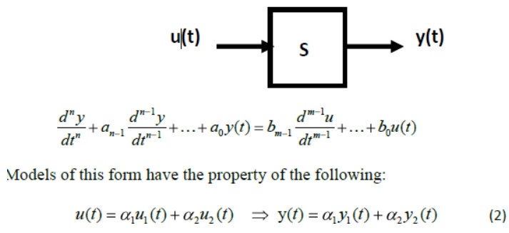
where, (y1, u1) and (y2,u2) each satisfies Eq,(1).
Model of the form of Eq.(1) is known as linear time invariant (abbr. LTI) system.
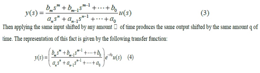
Assume the system is at rest prior to the time t0=0, and, the input u(t) (0 t <∞) produces the output y(t) (0 t < ∞), the model of Eq.(1) can be represented by a transfer function in term of Laplace transform variables, i.e.: